Network Analysis

Background

The objective of this exercise was to create an estimate of the cost each county in Wisconsin has to pay in order to transport frac sand from the mine to the nearest railroad terminal. Network analysis helped in determining which rail terminals were closest to each mine. This is one of the many practical ways network analysis can be utilized. 

Specifically, network analysis was run on the mines that were active, did not have loading stations on site, and that were at least 1.5 kilometers away from a rail station because then it was assumed the mine would directly load the sand onto the rails for transport. A python script was created to query the mines to produce a final feature class with all of the qualifying mines. 

Methods

Python 

The following python script shows the process of selecting mines based on certain criteria: 

• The mine must be active
• The mine cannot have its own loading station
• The mine has to be at least 1.5 kilometers away from a railroad terminal

Starting the script it was necessary to define the variables for the feature classes. For example, the variable set for the active_mines feature class was "act". Setting the variables ahead of time organizes the inputs and outputs while simplifying the script. 

The next step in python was to add field delimiters which provide the correct field information when creating an SQL statement. Field delimiters tell the program what field to search in. In this case "field1" dictated that when "field1" is coded in the script the field "SITE_STATU" in the attribute table is where the information will be found. 

Then, SQL statements were built to select active mines and only mines that did not have on-site loading stations. 

The SelectLayerByLocation tool was used to query out the mines that were within a distance of 1.5 kilometers of a rail station. 

Finally, the CopyFeatures tool was scripted to make a feature class for the mines that met all the criteria above. 

Figure 1. Python script used to select mines for network analysis. 

After the python script was successfully completed network analysis could be performed to find the quickest routes from the mines to the rail terminals. 

The network analyst toolbar was added to ArcMap. A streets network was added to the map along with the mines feature class (created from the python script) and the selected Wisconsin rail terminals feature class. In the network analyst toolbar, "New Closest Facility" was chosen to create the trucking routes. The mines were loaded into the analyst as incidents while the rail terminals were loaded as facilities. 

Solving the network produced overlapping routes, which is what is desired, compared to all of the routes combining when they reach a common point. This ensures that each route will have its own attributes and have a unique distance for each mine to the terminal. 

Model Builder

Model builder was used to find the distances (in miles) of each route and also to find the estimated cost each county to transport the frac sand. 

In model builder first the "Make Closest Facility Layer" tool was added with input of the streets feature class. The "Add Locations" tool was selected twice to make the mines the incidents layer and the rail terminals as the facilities. Then, the "Solve" tool ran to create the routes. Reference FIGURE to review the process. This produced the same result as above when the routes were solved for from the network analyst toolbar.  

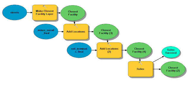
Figure 2. Model builder displaying the creation of routes from the mines to the closest rail terminal.

With the routes created it was necessary to add the routes to the database using the "Select Data" and "Copy Features" tools to produce a routes feature class. In order to determine the distance traveled and cost for each county, the "Intersect" tool was used to combine these features, however, first the routes and counties feature class were projected with UTM Zone 15N.

Figure 3. Model builder showing the projection and the intersection of the routes and counties feature classes.

Since the counties and routes were intersected it was possible to predict the distance traveled in each county and also the estimated cost to transport the sand. The "Summary Statistics", "Add Field", and Calculate Field" tools were used to create a table that included the distance traveled in miles and the cost for each county (Figure 4).  The distance traveled for each county was estimated with the "Calculate Field" tool and assigning the following equation [Shape_Length] * 100 (50 truck loads/year * 2 to account for the round trip) * 0.000621371 (miles in a meter). To estimate the costs for each county the equation was multiplied by 0.022, assuming it is roughly 2.2 cents for each truck per mile to transport the sand. 

Figure 4. Model builder displaying the use of various tools to create a table showing the cost and distance of the sand in each county. 

Figure 5 shows the final data flow model used from solving the network analysis to estimating the distance and cost of transporting sand for each county.

Figure 5. Final data flow model.

Results

Figure 6. Map displaying the routes from the mines to the rail terminals in Wisconsin.

Table 1. Results from the data flow model in adding fields to determine the total distance travel in miles and the cost estimate per county in dollars.

It is evident in Figure 7 that Chippewa, Eau Claire, and Barron counties have the highest estimate cost for transporting the sand. This could be attributed to the fact that in these counties the routes extend throughout most of the county. With more distance to be traveled in these counties the higher the cost would be to transport the material. Also, in Chippewa County and Eau Claire County multiple mine connect to a central rail terminal within the county (Figure 6), so there would be a lot of traffic associated to these routes as well. In the counties that experience little cost could be due to the fact that a mine or rail terminal lies right inside the county border, so the distance would be minimal for that county, as the case for Douglas County for example. 

Figure 7. Graph representing the estimated cost associated in each county for the transport of frac sand. 

Conclusion

To conclude using network analysis is a very powerful tool in answering many applied questions such as estimating the cost per county to transport a material. The ability to understand and successfully manage the data in network analysis and the data flow model to create the final output is crucial in determining accurate conclusions. This exercise challenged way the small details would affect the whole project, but helped me realize the applications network analysis can have.

Geocoding: Sand Mine Locations in Wisconsin

Background

The objective of this exercise was to be able to correctly identify roughly sixteen sand mines across the state of Wisconsin by geocoding. The data from this exercise originated from the Wisconsin Department of Natural Resources and were not in the correct format for geocoding initially. This lab served the purpose of introducing us to "imperfect data" and the errors that can occur if it is not properly formatted.

Geocoding: The process of assigning a physical location to an object, or correcting a previously set address. This is beneficial in analyzing data and specifically networking from one place to another.


Methods

As stated above the data provided to us from the Wisconsin DNR was not formatted in a way to be able to readily geocode the locations of the sandmines. The table contained one field for the address of a mine which cannot be read by the geocoding program. So, it was necessary to split the address into varying fields to separate street, city, state, county, etc. In addition to combining the whole address into one single field, the WDNR sometimes only provided the Public Land Survey description of the property. In that case a separate field was required to account for the description.

In the table I normalized I separated the orginal address field into ADDRESS_STREET, ADDRESS_CITY,  ADDRESS_STATE, ADDRESS_ZIP, and PLSS. This way the parts of the address were individual and could then be used to find that specific location on the map. In Table 1 you can see the result of my normalized table.

Table 1. Normalized table used to geocode the addresses of sand mines in Wisconsin. 

Once the table was normalized it could be added to ArcMap. The geocoding toolbar was turned on, and connected to ___________________. The interface automatically tried to match the addresses from the table to a location on the map.

Merge tool
I found the four other students that were assigned the same mines and used their shapefiles
-An error occured in merging because the zip code field different in one of the students tables, so I deleted that field because it was not needed. The field type was double and the student changed it to text.

Project
I projected the selected mines and my mines to State Plane System- Wisconsin Central: NAD_1983_2011_StatePlane_Wisconsin_Central_FIPS_4802

Select by attributes
To ensure the distance between my geocoded mines was matched with the same mine ID as the mines geocoded from my classmates, I created a new feature class for each of the sixteen mines my classmates geocoded. So, there were sixteen diferent feature classes, each representing one unique mine ID. Some feature classes only contained one mine, while others contained three or four depending on how the students geocoded or if they actually did the assignement.

As for comparing the distances between my mines and the actual location of the mine, I again created a separate feature class for each unique mine ID for the actual mine locations.

Near tool
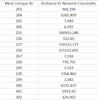
To succesfully get the distance to the closest mine the near tool was used. Some mines were way off their actual location and closer to a different mine, that is why the sixteen feature classes were created to identify the closest mine to each specific mine ID. When the near tool is run the distance will appear in the attribute table. But, since the each mine was run separately with this tool, only that specific mine ID distance will be correct. The tables (Table 2 and 3). below show the distances produced from running the near tool. The input features were my selected mines and the near features was the projected student mines or actual locations.

Table 3. Table showing the distance
from my geocodedmines to the actual 
locations of the mines. Unit in meters. 

Table 2. Table showing the distance from
my geocoded mines to theclosest 
geocoded mine of my classmates. 
Unit in meters. 

Results

Figure 1. Map comparing the mines I  geocoded to the mines geocoded by classmates, and the actual location of the mines.  

From the map it appears my geocoded mines were not too far off from the actual location of the mines, however, the closest one of my mines was to the actual location is 260 meters. In fact, three mines 237, 238, and 235 were geocoded in the same location northeast of their actual locations. The geocoding toolbor automatically assigned the mines to this location, and I made the mistake of not correcting those locations. Also, I confused mine 269 for mine 270 and vice versa. I noticed this while running the near tool when the table produced a closer distance for another mine than the one I was searching for. This could be attributed to not reading the address correctly and that there were two mines close by!

In reviewing  locations where my mines were far from the actual location I noticed that some of the mines were classified as inactive, which could be a reason to why the locactions did not match. The mines that did not appear on the basemap or google earth were the hardest to identify because there was no way of telling where the mines driveway was. 

Conclusion

This exercise clearly demonstrated the importance of normalizing data and being aware of the errors possible throughout the whole geocoding process. According to Lo ___________, there are three types of error: Gross, Systematic, and Random. During this exercise many errors affected the how the mines were geocoded. 

Gross error: the user makes a mistake in managing the data. A great example of this was stated above for mines 235, 237, and 238 that were all geocoded in the same location. That was an oversight by me to not go in and manually change where the mine was. 

Systematic error: errors attributed to bias in measurements of the user and faulty equipment to name a few. In this exercise an example of systematic error was my personal mine locations differed (in some cases a lot) from the mines of my classmates. We each had our own bias as to we thought the coordinate of the mine should be located. Therefore, we had varying data. 

Random error: errors due to the limitation of the equipment taking the measurements for data collection. 

Specifically the some errors in this exercise could have been easily avoided. First, if all of the students were given a normalized addresses in the attribute table that would avoid any mistakes from trying to transform the table to work with the data. Second, more guidelines as to where the coordinate should be placed in relation to the mine would help in eliminating some human bias. In conclusion, this exercise demonstrated the purpose of preparing data ahead of time, especially when the data will be distributed to a team to work on.